4 检验的功效与渐进相对效率

先载入一些包：

library(tidyverse)

4.1 检验的功效

利用统计模拟的方法，比较单样本位置检验中不同检验方法的功效。

4.1.1 假设检验问题

随机变量\(X_1,\cdots,X_n\)是来自连续分布总体\(F(x-\theta)\)的样本，函数\(F(t)\)关于0点对称。检验假设： \[ H_0:\theta=0\qquad v.s. \qquad H_1:\theta>0 \]

4.1.2 检验方法

T检验。检验统计量为： \[ T=\frac{\bar X}{S/\sqrt{n}} \]

其中，\(\bar X\)为样本均值，\(S\)为样本标准差。拒绝域为\(T\ge t_{n-1}(1-\alpha)\)

符号检验。检验统计量为： \[ S^+ = \sum_{i=1}^n\psi(X_i) \] 拒绝域为\(S^+\ge b(1-\alpha,n)\).
符号秩检验。检验统计量为： \[ W^+ = \sum_{i=1}^n\psi(X_i)R_i^+ \] 拒绝域为\(W^+\ge w(1-\alpha,n)\)。

4.1.3 实验分布

选择典型的常用对称分布，分别为[-1,1]上均匀分布、正态分布、Logistics分布、Cauchy分布。

ggplot()+
  geom_function(aes(colour = "unif"),fun = dunif,args = list(min=-1,max=1))+
  geom_function(aes(colour = "norm"),fun = dnorm)+
  geom_function(aes(colour = "logistic"),fun = dlogis)+
  geom_function(aes(colour = "cauchy"),fun = dcauchy)+
  lims(x=c(-4,4))+
  ggtitle("各分布密度函数图")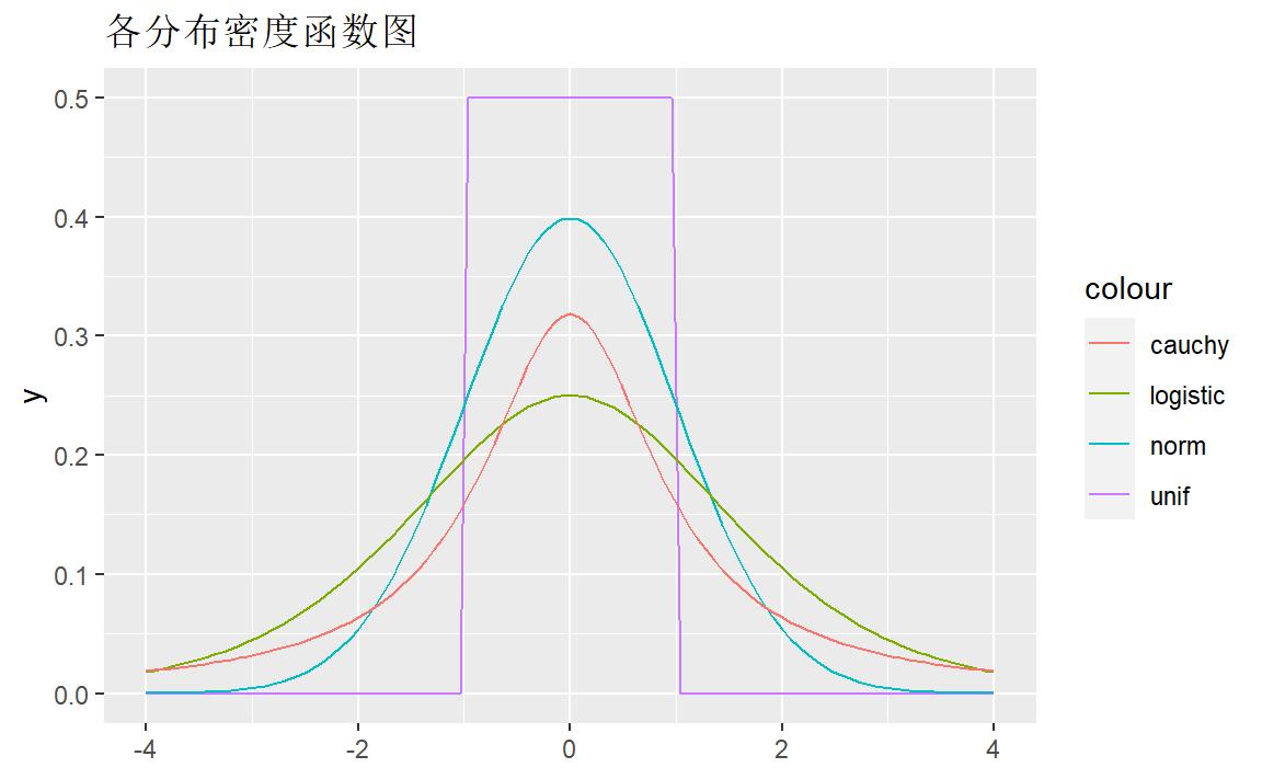

4.1.4 统计模拟

一些预定参数：

对固定分布\((\theta,F)\)产生样本值1000次，每次100个样本；
显著性水平\(\alpha\)取0.05。

# 定义带参数的均匀分布作为新函数
runif_new <- function(n){
  runif(n,min = -1,max = 1)
}

# 检验功效函数
testpower <- function(theta,funcs,n=100,times=1000,alpha=0.05){
  library(tidyverse)
  
  s <- funcs(n*times)+theta  # 产生样本
  s <- matrix(s,nrow = times) # 每行为一组样本
  # T检验功效
  p <- apply(s,1,t.test,alternative = "greater") %>% 
    map(~.$p.value) %>% 
    unlist()
  pt <- mean(p<alpha)
    
  # 符号检验
  # 求大于0个数
  postn <- function(x){
    sum(x>0)
  }
  # 求等于0个数
  zeron <- function(x){
    sum(x==0)
  }
  s1 <- apply(s,1,postn)
  s2 <- apply(s,1,zeron)
  p <- map2(s1,n-s2,binom.test,p = 0.5,alternative = "greater") %>% 
    map(~.$p.value) %>% 
    unlist()
  ps <- mean(p<alpha)

  # 符号秩检验
  p <- apply(s,1,wilcox.test,alternative = "greater",mu=0) %>% 
    map(~.$p.value) %>% 
    unlist()
  pw <- mean(p<alpha)

  l <- list(pt=pt,ps=ps,pw=pw)
  
  l
}

对均匀分布：

theta <- seq(0,0.7,by = 0.1)
map(theta,testpower,funcs=runif_new)->ln
df <- data.frame(matrix(unlist(ln), ncol=3,byrow = TRUE))
df %>% 
  rename(pt=X1,ps=X2,pw=X3) %>% 
  ggplot(aes(x=theta))+
  geom_line(aes(y=pt,color="T检验"))+
  geom_line(aes(y=ps,color="符号检验"))+
  geom_line(aes(y=pw,color="符号秩检验"))+
  labs(title = "均匀分布",y="功效",color="检验方法")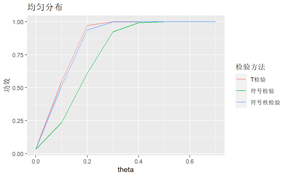

T检验方法比符号秩检验方法稍好，符号检验方法较差。

对正态分布：

theta <- seq(0,0.8,by = 0.1)
map(theta,testpower,funcs=rnorm)->ln
df <- data.frame(matrix(unlist(ln), ncol=3,byrow = TRUE))
df %>% 
  rename(pt=X1,ps=X2,pw=X3) %>% 
  ggplot(aes(x=theta))+
  geom_line(aes(y=pt,color="T检验"))+
  geom_line(aes(y=ps,color="符号检验"))+
  geom_line(aes(y=pw,color="符号秩检验"))+
  labs(title = "正态分布",y="功效",color="检验方法")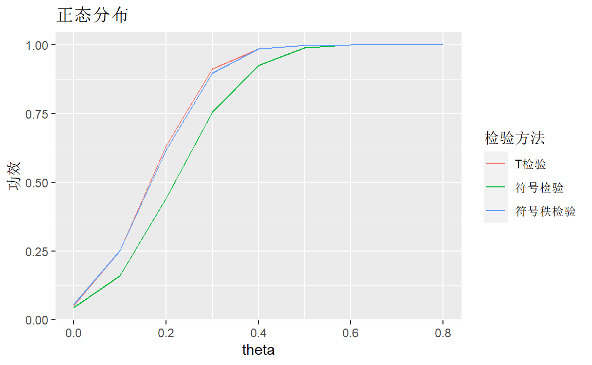

T检验方法比符号秩检验方法稍好，符号检验方法较差。

对Logistics分布：

theta <- seq(0,1.5,by = 0.1)
map(theta,testpower,funcs=rlogis)->ln
df <- data.frame(matrix(unlist(ln), ncol=3,byrow = TRUE))
df %>% 
  rename(pt=X1,ps=X2,pw=X3) %>% 
  ggplot(aes(x=theta))+
  geom_line(aes(y=pt,color="T检验"))+
  geom_line(aes(y=ps,color="符号检验"))+
  geom_line(aes(y=pw,color="符号秩检验"))+
  labs(title = "Logistic分布",y="功效",color="检验方法")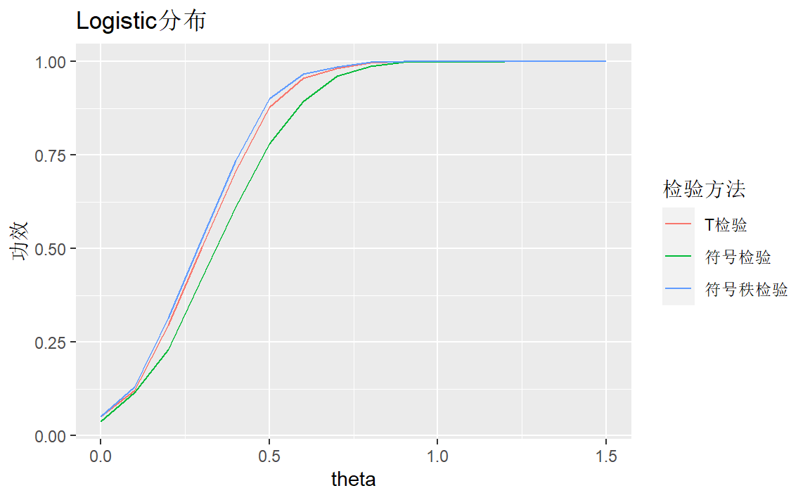

三种检验方法比较接近，符号秩检验方法稍好。

对Cauchy分布：

theta <- seq(0,1.5,by = 0.1)
map(theta,testpower,funcs=rcauchy)->ln
df <- data.frame(matrix(unlist(ln), ncol=3,byrow = TRUE))
df %>% 
  rename(pt=X1,ps=X2,pw=X3) %>% 
  ggplot(aes(x=theta))+
  geom_line(aes(y=pt,color="T检验"))+
  geom_line(aes(y=ps,color="符号检验"))+
  geom_line(aes(y=pw,color="符号秩检验"))+
  labs(title = "Cauchy分布",y="功效",color="检验方法")

符号检验方法较好，T检验方法很差。

所以，如果我们对\(H_1\)下的分布有一定的先验知识：峰度等，可以选择适宜的检验方法，也可以通过估计来粗略得到分布的峰度、偏度等等。