第二个模型的部分代码
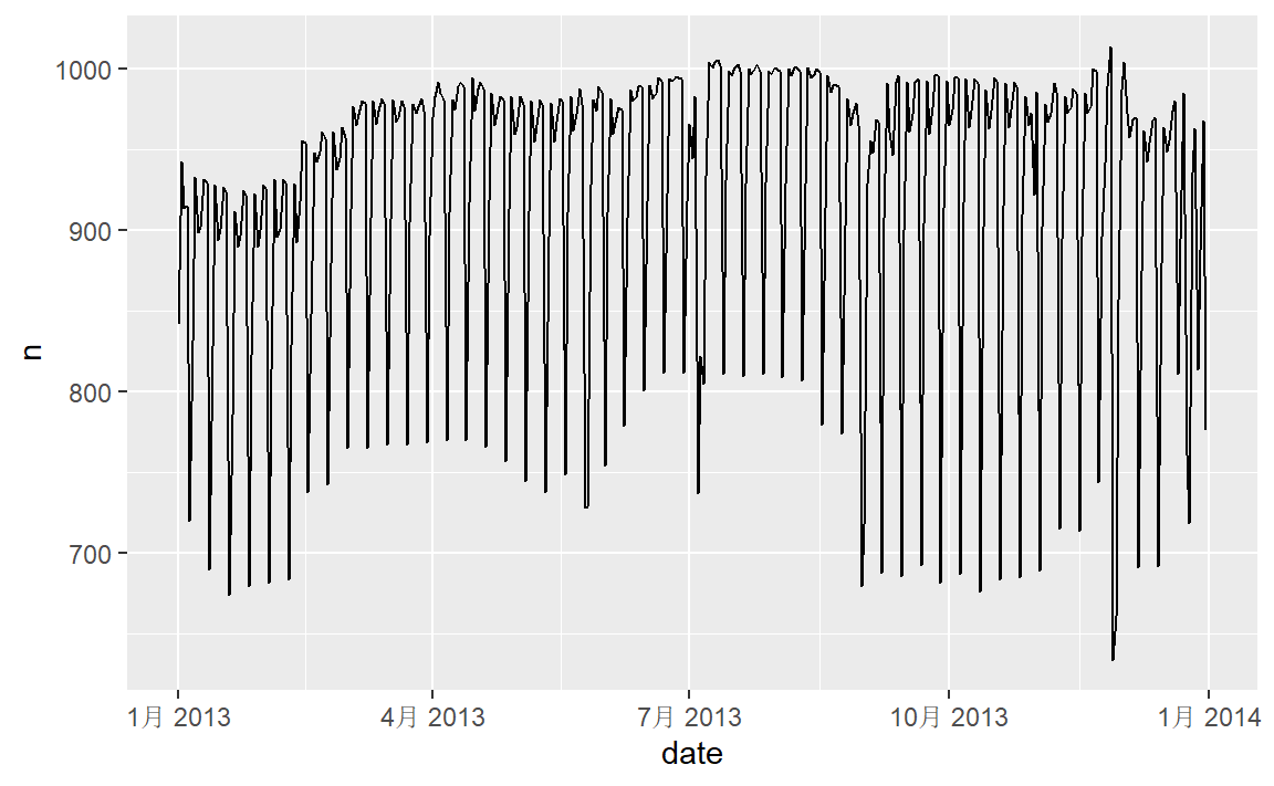
# 每天的航班数量
daily <- flights %>%
  mutate(date = make_date(year, month, day)) %>%
  group_by(date) %>%
  summarize(n = n())
#> `summarise()` ungrouping output (override with `.groups` argument)
daily
#> # A tibble: 365 x 2
#>   date           n
#>   <date>     <int>
#> 1 2013-01-01   842
#> 2 2013-01-02   943
#> 3 2013-01-03   914
#> 4 2013-01-04   915
#> 5 2013-01-05   720
#> 6 2013-01-06   832
#> # ... with 359 more rows
ggplot(daily, aes(date, n)) +
  geom_line()
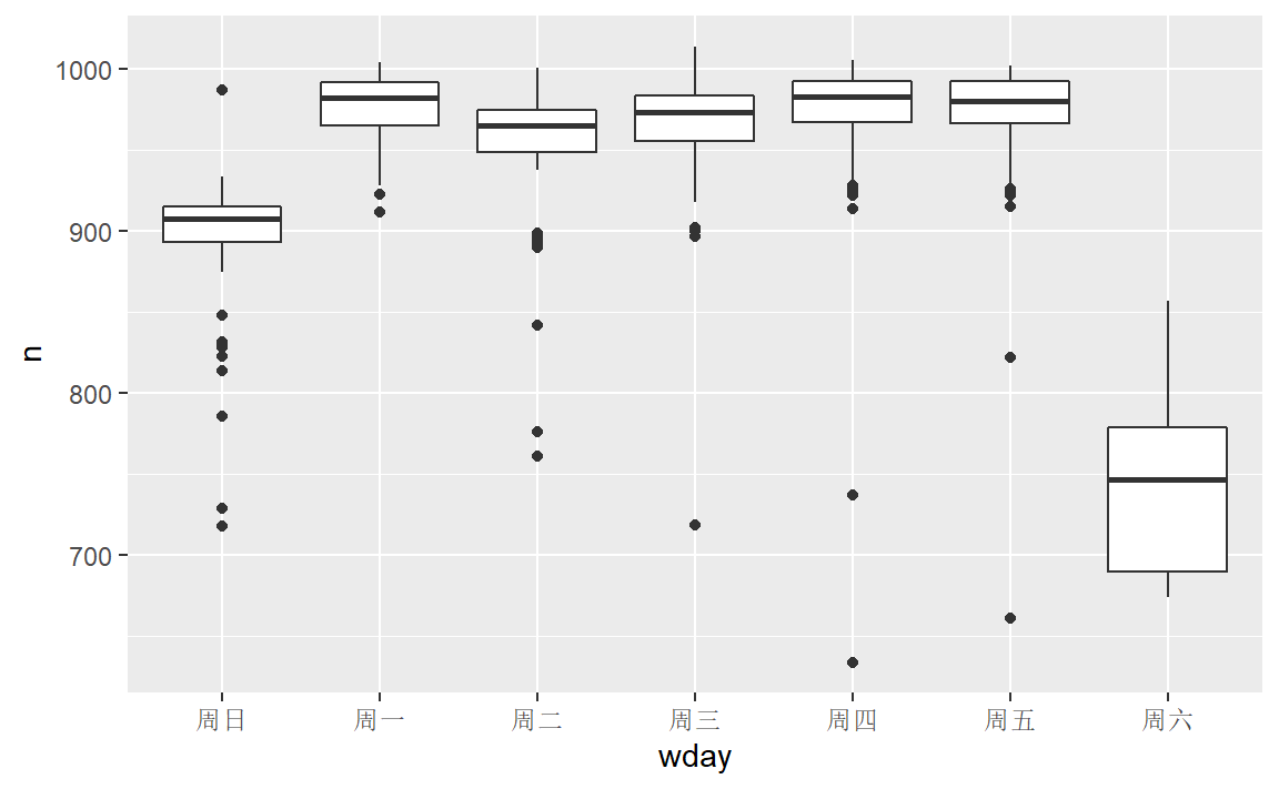
daily <- daily %>%
  mutate(wday = wday(date, label = TRUE))  # 添加星期变量
# 绘制星期与航班数量的箱线图
ggplot(daily, aes(wday, n)) +
  geom_boxplot()
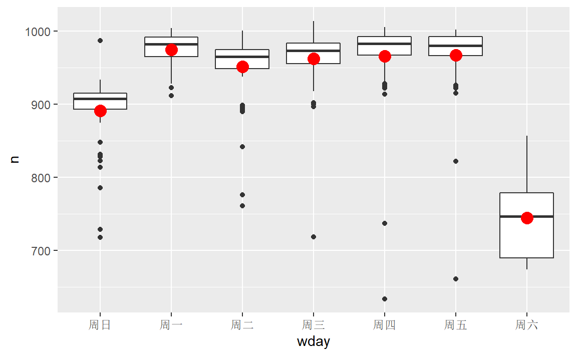
mod <- lm(n ~ wday, data = daily) # 拟合模型

grid <- daily %>%
  data_grid(wday) %>%
  add_predictions(mod, "n")   # 添加预测值

ggplot(daily, aes(wday, n)) +
  geom_boxplot() +
  geom_point(data = grid, color = "red", size = 4)  # 将预测值放在上图中
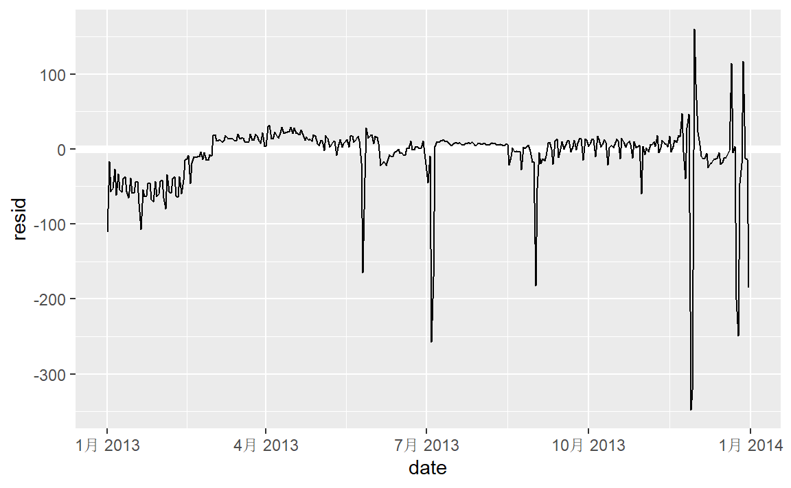
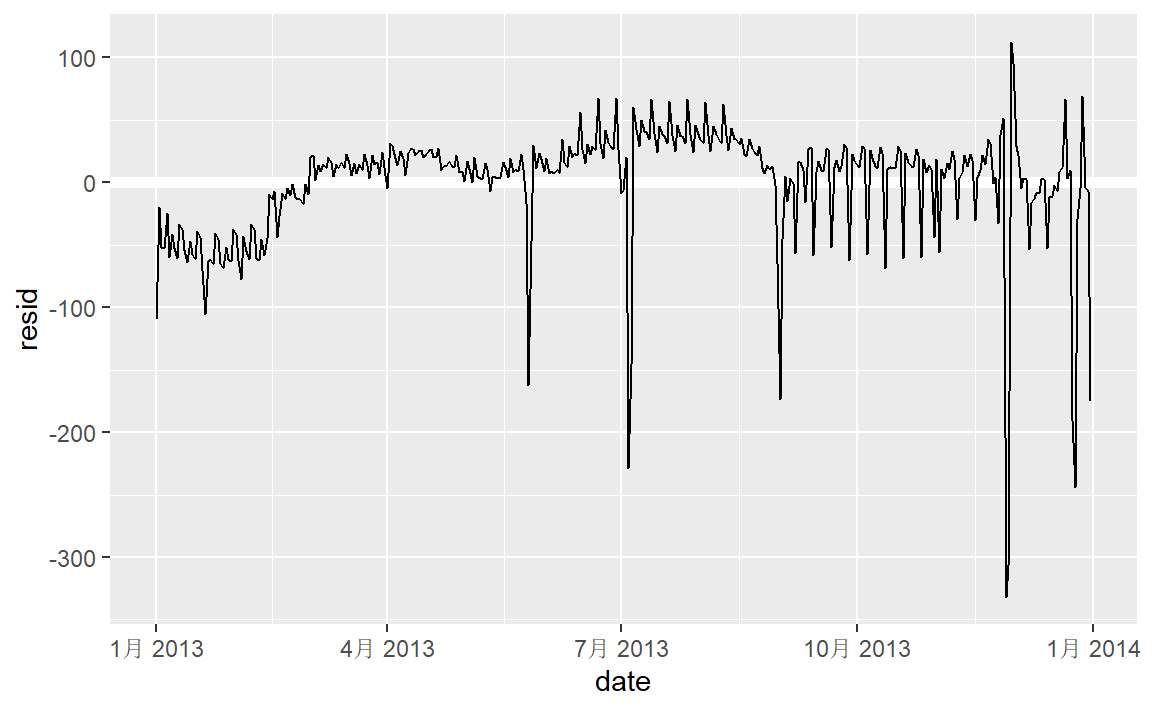
daily <- daily %>%
  add_residuals(mod)  # 添加残差
daily %>%
  ggplot(aes(date, resid)) +
  geom_ref_line(h = 0) +
  geom_line()
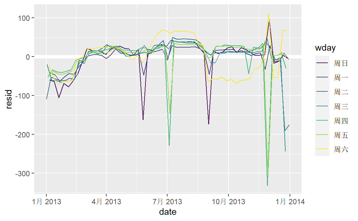
ggplot(daily, aes(date, resid, color = wday)) +
  geom_ref_line(h = 0) +
  geom_line()
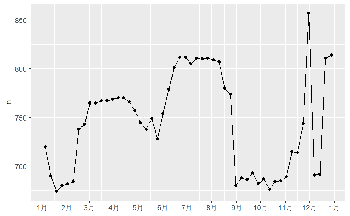
daily %>%
  filter(wday == "周六") %>%
  ggplot(aes(date, n)) +
    geom_point() +
    geom_line() +
    scale_x_date(
      NULL,
      date_breaks = "1 month",
      date_labels = "%b"
    )
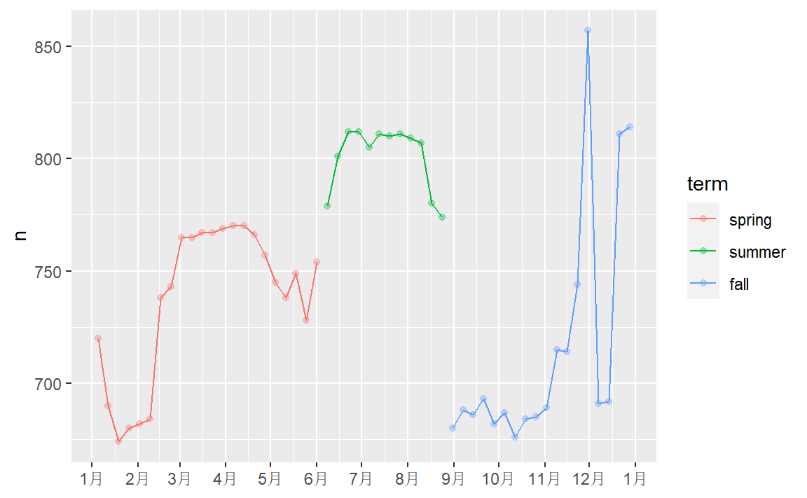
term <- function(date) {
  cut(date,
    breaks = ymd(20130101, 20130605, 20130825, 20140101),
    labels = c("spring", "summer", "fall")
  ) # cut将日期转为因子
}
daily <- daily %>%
  mutate(term = term(date)) # 划分日期为季节
daily %>%
  filter(wday == "周六") %>%
  ggplot(aes(date, n, color = term)) +
  geom_point(alpha = 1/3) +
  geom_line() +
  scale_x_date(
    NULL,
    date_breaks = "1 month",
    date_labels = "%b"
  )  # 设置x轴的时间标签
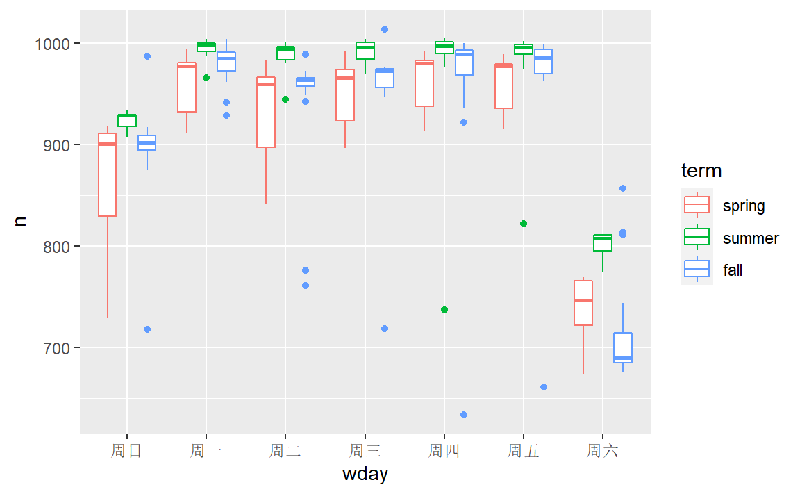
daily %>%
  ggplot(aes(wday, n, color = term)) +
    geom_boxplot()
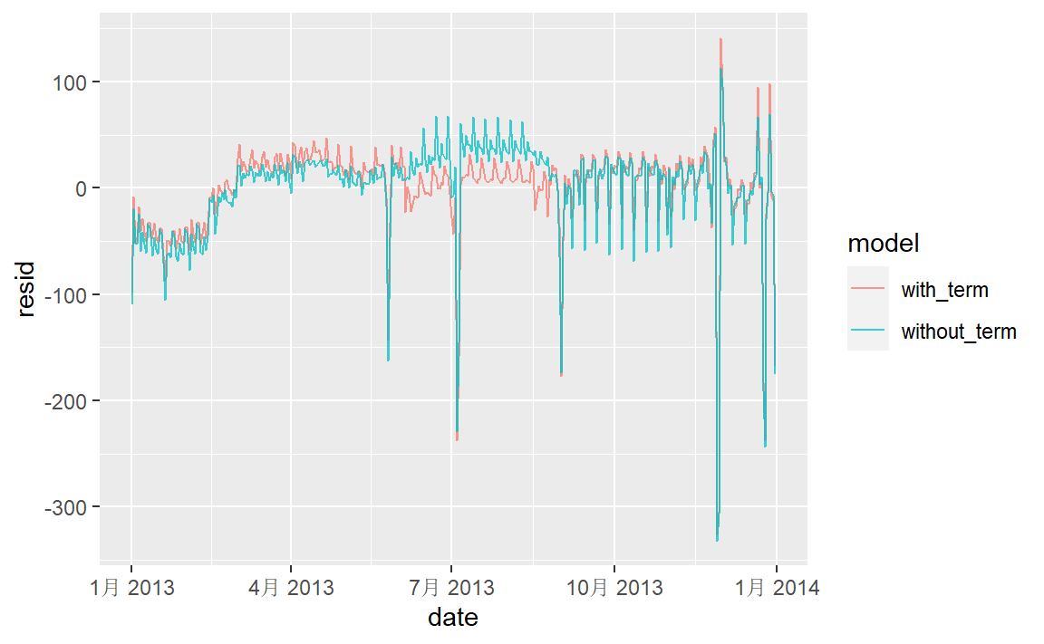
mod1 <- lm(n ~ wday, data = daily)
mod2 <- lm(n ~ wday * term, data = daily)

daily %>%
  gather_residuals(without_term = mod1, with_term = mod2) %>%
  ggplot(aes(date, resid, color = model)) +
    geom_line(alpha = 0.75)
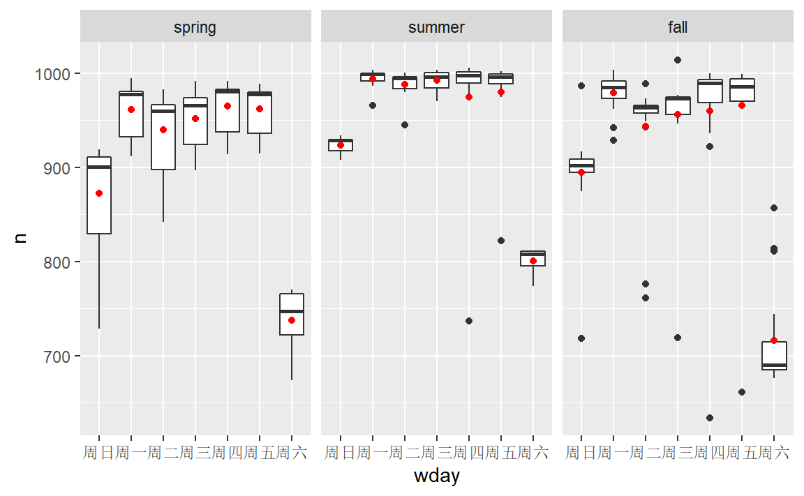
grid <- daily %>%
  data_grid(wday, term) %>%
  add_predictions(mod2, "n")

ggplot(daily, aes(wday, n)) +
  geom_boxplot() +
  geom_point(data = grid, color = "red") +
  facet_wrap(~ term)
# 尝试稳壮的线性回归
mod3 <- MASS::rlm(n ~ wday * term, data = daily)

daily %>%
  add_residuals(mod3, "resid") %>%
  ggplot(aes(date, resid)) +
  geom_hline(yintercept = 0, size = 2, color = "white") +
  geom_line()